

Greetings to all eager learner!!!
Now a days all of us are aware of how data science is trending in the market. Most of us are aware about machine learning concepts also. How someone can minimize the work cost by using Machine learning algorithm. But before moving to Machine learning algorithm it is mandatory to understand basics of statistics. Basics of statistic is the core of machine learning algorithm, no matter what tool is been used. There are many tools, scripting-programming languages like R, Python, SAS, Watson, Power BI, Tableau etc. having libraries or packages based on statistics.
This blog will help you to understand how concepts of statistics enhance accuracy in the machine learning algorithm.
So here we are starting from very basic concept that is Population and sample with R programming. Sampling plays a major role in machine learning algorithm.
For Free, Demo classes Call: 8983120543
Registration Link: Click Here!
DATA SAMPLING & DISTRIBUTION
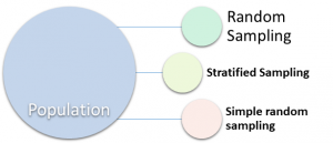
Population: The larger data set. Size of Population is denoted by N.
Sample: Subset of Population is Sample.
Random Sampling: Collection of random elements from population is called random sampling. In this process every element has equal chance of being chosen at each selection.
Stratified sampling: Dividing population into subgroup or strata. Data is randomly collected from each strata and group
Simple random Sampling: Collection of the data from random sample without stratifying the population
Sample bias: Sample which is not giving clear information about population is called sample bias. It is misrepresenting the population.
Quality of sample is more important than quantity of the sample. The quality of the data refers to consistency of the format, accuracy, cleanliness and completeness of each individual point in the given data.
Bias: Error caused due to sampling process. There is difference between error due to random chance and error due to bias.
Sample Mean Vs. Population Mean
X: is mean of sample.
µ: is mean of Population.
Sampling Distribution of a statistic:
Data distribution can be defined as the frequency distribution every data point in the data set.
Classical statistics helps to define some inference based on small sample. The same inference can be applicable to large population.
Randomization and Sampling distribution using R code
sample ( x , size, replace = FALSE)
sample (1 : 10)
This gives all 10 numbers in random order
sample (1 : 10 , 3)
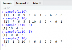
code 1
sample() is the function in R language to create sampling of the numbers. Here in the above code we have passed the range from 1 to 10. 3 is the set of numbers in sample. Hence output of the code is as mentioned below:
For Free, Demo classes Call: 8983120543
Registration Link: Click Here!
4 , 8 , 6
This output varies on each and every execution.
Mean: Mean is the average of the data. That is summation of all points divided by total number of units.
For the data point 1 to 10 mean is calculated as mentioned below:
Add = 10 + 9 + 3 + 4 + 5 + 6 + 7 + 8 + 2 + 1 = 55
Mean = 55 / 10 = 5.5
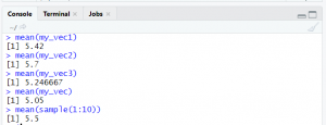
So for population mean is not going to change and it will be same at any point of time. The same is shown in below mentioned figure-code1. First two line is the execution of mean of sample. However that is not the case with sample. For random sampling, mean ( ) is changing based on selection of data points and size of the sample.
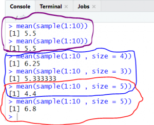
code 2
Mean for sample with size 4 is 6.25.
Mean for sample with size 3 is 5.33.
Mean for sample with size 5 is 4.4 at first time and 6.8 at second time. Now the question is, Why mean is different though size is same? This is because on each and every execution selection of data point is different for sample.
Trimmed MEAN:
Average of data points after trimming off sorted data points from both sides.
Equation of trimmed mean is
Weighted MEAN:
Median and Outlier:
The next example is how mean of sample will help to work on population.
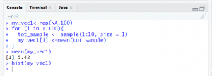
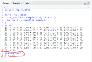
rep(NA, 100) : rep() function is used to create vector of the same value. Hence my_vec variable is holding hundred NA values.
Code3 is an example to create sample of random 4 numbers within 1 to 10 for 100 times. At each execution numbers appearing in the sample varies. Mean of all hundred sample is stored in variable my_vec1
hist ( my_vec ): hist is the function to plot histogram in R. Histogram is showing the frequency distribution of each and every point.
code 3
The above example shows that we have created sample for only one number. And the histogram of the mean created based on the sample is shown as below:
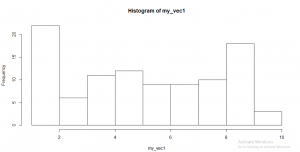
histogram 1
Now the next step is change the size to 2.
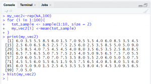
code 4
Histogram for sample size 2 is shown in fig
histogram 2
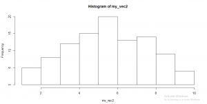
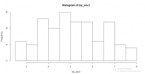
Change size to 3 now :
code 5

histogram 3
For Free, Demo classes Call: 8983120543
Registration Link: Click Here!
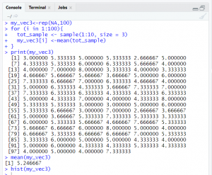
Code6 is the example where we are creating sample of random 4 numbers within 1 to 10 for 100 times. At each execution numbers appearing in the sample varies. Mean of all hundred sample is stored
code 6
Observation: mean of sample mean for any sample with any size is approximately equal to mean of population. Refer code7 my_vec1
code 7
histogram 4
What is Bootstrap?
One of the easiest and effective process for sampling distribution is the bootstrap sampling. This is just a process to replace of one observation with another. If the sample size is less than 30 we can use bootstrap sampling. On other hand if sample size is greater than 30 we can use CLT (Central Limit theorem). Bootstrap sampling helps to determine sampling distribution without CLT.
Bootstrap example in R:
Suppose we got prizes of ten different pen.
5, 15, 6, 8, 20, 5, 18, 15, 16, 2
Calculations are as mentioned below:
- calculate mean of the data
Mean is 11
- standard deviation of the data 6.44
- standard error of the data 2.03
Standard error is calculated as standard deviation of the sample data divided by square root of number of samples.
√n
For Free, Demo classes Call: 8983120543
Registration Link: Click Here!
Bootstrap sample:
A sample created with replacement from an observed data set.
Resampling:
The process of taking repeated samples from observed data; includes
both bootstrap and permutation (shuffling) procedures.
The algorithm for a bootstrap resampling of the mean is as follows, for a
sample of size n:
- Draw a sample value, record, replace it.
- Repeat n times.
- Store the mean of the n resampled values.
- Repeat steps 1–3 R times.
- Use the R results to:
- Calculate their standard deviation (this estimates sample mean standard error).
- Produce a histogram or boxplot.
- Find a confidence interval.
##################################
Central Limit Theorem (CLT)
The central limit theorem is tendency of sampling distribution to take on a normal shape as sample size increases. The central limit theorem is an important technique in traditional statistics texts. Based on Central limit theorem analysis of hypothesis tests and confidence intervals can be done. Distribution of collection of all Mean ( ) drawn from each and every sample shows normal distribution. The next blog we will focus on Central limit theorem.
Author:
Helwade, Amrita
Designation: Software Trainer
Company: Seven Mentor Pvt. Ltd.
Call the Trainer and Book your free demo Class for now!!!

© Copyright 2019 | Sevenmentor Pvt Ltd.